
Heat Spreading Calculations Using Thermal Circuit Elements
Bruce Guenin, Associate Technical Editor
Introduction
In electronics cooling applications, there are numerous changes of scale from the chip level to the system level. This is characteristic of the signaling, power, and thermal infrastructures in
electronic systems. Because of this, it is inevitable that the heat flow from the smallest scale to the largest be accompanied by heat spreading. This column explores one of the many possible heat spreading
situations encountered in electronics cooling.
This exercise is also intended to serve as an example of a more general procedure of representing a complicated heat flow pattern with a number of thermal circuit elements, each appropriate for different
regions of the heat flow pattern. When linked into an appropriate thermal network, these thermal elements can be used to predict heat source temperatures in a large variety of situations.
Description of Problem
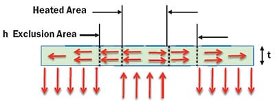
The particular situation of interest is that depicted in Figure 1. It consists of a plate, centrally heated by a uniform heat flux and uniformly cooled in its peripheral region. The
boundaries between these various regions are square.
 TITLE=”2008_Aug_CC_Figure01″>
Figure 1. Heat flow patterns in a square plate having central heating and peripheral cooling.
The heat flow path can be divided into three distinct regions
One example of this would be the heat spreader on top of a cavity-type BGA package. The heat is injected into the center of the heat spreader by the die and extracted from its periphery by the
package laminate, which, in turn, would transmit the heat to a PCB through the solder ball interconnection between them [1].
Note that this situation is different from a more typical one with heat injected into one side of a plate and extracted at constant h from the entire reverse side. There is a well-known approach to this
particular problem [2].
Finite Element Analysis Solution
As has been the practice in previous columns, a commercially available Finite Element Analysis (FEA)
tool has been used to produce thermal solutions for the situations of interest [3]. Since the FEA mesh was appropriately refined to obtain a fully converged solution, it is considered to be “exact.”
Table 1 lists the physical parameters characterizing the situation analyzed and the particular values used in the simulations. They were chosen to be representative of values used in typical electronics
cooling applications. The parameters, t, WHeat, Wh_Excl, and h were varied to test the accuracy of the analytical solution.
Table 1. Parameters and Values Used in Simulation.
 |
The values of h chosen for this exercise are much higher than those that would result from direct convective cooling of the plate with air. However, in a typical electronics cooling environment, values of
this magnitude could be achieved by conduction heat transfer from the plate to a component with an extended surface, such as a heat sink.
Equation 1 is used to calculate the source-to-ambient thermal resistance.
 |
Since in the simulation, TAmb and P were conveniently chosen to be 0�C and 1 W, respectively, ΘSA will simply equal the calculated value of TSource. This will not have an effect on the generality of these
results since there are no temperature-dependent heat transfer processes assumed in this model, making ΘSA independent of P. The following analysis will consider values of ΘSA based on both the peak
source temperature ( ΘSA, Peak) and the average source temperature ( ΘSA, Avg), since each are of value to the thermal engineer, depending on the situation.
Figure 2 displays various outputs of the model. The graph in Figure 2a plots the calculated values of ΘSA, Avg versus Wh_Excl, with each curve representing constant values of the parameters h, WHeat,
and t. For each curve, the calculated values vary over a large range. This is mainly due the variation in Wh_Excl and its resultant effect on the area over which h is applied (79 to 1479 mm²
). The choice for h (500 or 5000 W/m²K) was second in significance in determining ΘSA. The value selected for t (0.1 or 1
mm) was third. The graph in Figure 2b plots the plate temperature versus its position either along the x-axis or the diagonal for three of the cases evaluated. In one case the temperature profiles for the
two paths overlap. In the other two they differ. This behavior will be addressed again in the context of the error discussion for the analytical method.
 |
Figure 2. Results of FEA calculations.
Note, in these specific examples, Case #19 for the 0.1 mm thickness shows a much larger temperature difference between the center and the edge of the plate than do the other two cases at
the 1.0 mm thickness. Furthermore, for Cases #6 and #9, each with the higher value of h = 5000 W/m²K, the temperature at the edge of the plate is very close to Tamb. In Case #1, on the other hand,
h = 500 W/m²K, and there is over a 1�C temperature difference. Note: for Case #1, Wh_Excl = 11mm, which is associated with an area of h application of 1479 mm²
, the maximum value considered. As this area decreases for larger values of Wh_Excl the temperature difference increases proportionately.
Figures 2c and 2d contain the calculated thermal contour plots calculated for Cases #1 and #19. The contours near the source region manifest a circular symmetry in Case #1 but more of a square
symmetry for Case #19. This is consistent with the temperature profiles in Figure 2b.
The results of all the FEA simulations are presented in Table 2 along with the results of the analytical calculations.
Table 2. Comparison of FEA and Analytical Results.
 |
Thermal Circuit Element Approach
The heat flow pattern described above can be represented by three thermal circuit elements, with each corresponding to one of the three regions described above.
It is a fact of life that closed form solutions for heat flow can be derived much more easily for geometries with circular symmetry than with square symmetry. We take advantage of this fact in the
expressions presented below. In doing so, we convert the width, W, of a region boundary to a radius, R, of a circular region of the same area; i.e.:
SRC=”http://s3.electronics-cooling.com/legacy_images/2008/08/2008_Aug_CC_Eq_p11.jpg” VSPACE=0 HSPACE=0 ALIGN=”TOP” border=0 ALT=”2008_Aug_CC_Eq_p11″ TITLE=”2008_Aug_CC_Eq_p11″>
The appropriate expressions are indicated below for each of the three regions:
 |
where α = (Nh/κt)1/2, N is the number of surfaces cooled by h (1 or 2), and I0 , I1 (K0 , K1) are
modified Bessel functions of the 1st (2nd) kind, order 0 and 1. (Note: Bessel functions I0 , I1 , K0 , and K1 are represented in popular spreadsheets as: BESSELI(X,0), BESSELI(X,1), BESSELK(X,0), and
BESSELK(X,1), respectively.) These somewhat intimidating functions have been put to use in previous installments of this column [5, 6].
Finally, since the overall heat flow represents a simple series circuit, ΘSA, Avg and ΘSA, Peak can
calculated by simply summing up the calculated values of the three appropriate resistances:
 |
The calculated values of ΘSA, Avg and ΘSA, Peak are presented along with the associated error when
compared with the FEA results. In most cases the error is less than 1%. However, in a few of the cases, the error is larger, up to 4.6% for ΘSA, Avg and 2.4% for ΘSA, Peak
To rationalize this error, one need only take a second look at Figure 2b. Cases #1, #6, and #19 had error values of 0.4, 2.1, and 4.6%, respectively. In Case #1, the temperature profiles along the axis
and diagonal are very nearly the same. This means that, in spite of the square symmetry of the plate shape and the heating and cooling loads, the temperature profile exhibits a circular symmetry. Hence,
in this case, the actual heat flow is consistent with that assumed in using the above equations. This is clearly not the situation for Cases # 6 and #19. Here, the larger h value of 5000 W/m²K produces a
more pronounced thermal gradient and more forcefully imposes the square symmetry of the problem geometry on the heat flow.
As a general rule, the more closely the heat flow pattern implicit in the derivation of the chosen thermal circuit elements corresponds to the actual heat flow, then the more accurate will be the
temperature prediction.
The use of thermal circuit elements to approximate a complicated heat flow bears a resemblance to the practice in Computer Aided Design (CAD) of using primitives, such as rectangular blocks, cylinders,
and spheres, to construct more complicated shapes. However, the use of thermal circuit elements is more subtle, since not only the geometry but also the thermal gradients must be carefully considered
when choosing the proper elements for a problem.
Conclusions
An analytical method to predict the thermal resistance of a plate with central heating and peripheral
cooling has been demonstrated. According to this method, each of three regions of the heat flow is represented by an appropriate thermal circuit element. The accuracy of this method was associated
with the fidelity of the flow as represented by the thermal circuit elements compared with the actual heat flow.
References
Conference on Thermal Phenomena in Electronic Systems (iTherm), May, 1994, pp. 50-61.


Leave a Reply