Introduction
A transient thermal characterization, also known as a thermal survey, aims to characterize the location of greatest thermal inertia within a hardware system—that is, the location with the slowest temperature response to a given environmental stimulus. This manuscript outlines a methodology for developing a finite difference numerical model of a three-resistor, four-node series network that characterizes the transient thermal response of a hardware system. A numerical model of the system was calibrated to experimental temperature data and validated with commercial software. The model outlined herein is easy to implement on a spreadsheet. The mathematical and numerical framework was previously described in Ref. [1].
The hardware system characterized herein was comprised of multiple circuit boards arranged in a tightly spaced parallel layout. Each circuit board was mounted to a thin aluminum coldplate with internal channels designed for single-phase liquid flow-through cooling. All circuit board and coldplate assemblies were mounted to a larger circuit board that was in turn mounted to a large aluminum baseplate, which served as the liquid distribution manifold for the system. The baseplate assembly was enclosed by aluminum walls that served as the housing of the hardware system. Therefore, the hardware system was comprised of various, multi-level internal assemblies.
| Nomenclature # | Definition |
|---|---|
| NA | Ambient node (boundary condition) |
| N1 | Hardware exterior node |
| N2 | Hardware interior node with intermediate inertia |
| N3 | Hardware interior node with greatest thermal inertia |
| Tn | Temperature of node n |
| Cn | Thermal capacitance for node n |
| Rnm | Thermal resistance between nodes n and m |
| ̇Qn,D | Heat dissipation rate for node n |
| ̇Qnm | Heat transfer rate between nodes n and m |
Nodal Network Representation
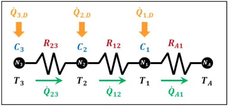
As illustrated in Figure 1, a hardware system can be approximated as consisting of three nodes (N1, N2, and N3) according to the lumped capacitance methodology [2]. Node N1 represents the surfaces of the hardware that are in direct contact with the ambient environment node NA and therefore exhibits the fastest response to the ambient environment (i.e., has the least thermal inertia). Node N2 represents an intermediate location within the hardware. Node N3 represents the interior location with the greatest thermal inertia, giving it the slowest temperature response to the ambient environment. Each node is characterized by a thermal capacitance, Cn, while each resistor-node pair is characterized by a ther al resistance, Rnm. Each node exhibits a heat dissipation rate, QD, which may be zero. Each node is assumed to be at a uniform temperature, consistent with the lumped capacitance method. Internodal heat transfer is marked by convection between the hardware and ambient nodes (i.e., RA1) and by heat conduction within the hardware (i.e., R12 and R23). Internal convection and radiation are assumed to be negligible within the hardware, which is usually the case in electronics packaging applications due to the tight spacing within small form factors and relatively low temperatures.

Experimental Data Collection
The first step in performing a transient thermal characterization was to experimentally collect temperature data from the interior of the hardware. Since the physical location of greatest thermal inertia may not always be intuitive or known a priori, it is recommended that the temperatures of multiple locations, any of which may possibly represent the location of greatest thermal inertia within the hardware, be monitored.
For this test, the hardware was disassembled and thermocouples were affixed to various internal locations. Kapton tape, a thermally and electrically non-conductive adhesive with minimal residue, is usually sufficient for quick tests as long as heat transfer is minimized across the attachment material [3]. Then, the instrumented hardware was reassembled and placed inside an environmental temperature chamber. Next, temperature data were recorded while the chamber was brought to a temperature extreme. The hardware was tested in a “dead mass” condition, which signifies that all electronics in the hardware were off and therefore exhibited zero heat dissipation and that the hardware had no active cooling during testing. Fluid channels in the coldplates and baseplate were devoid of liquid coolant, in order to characterize only the hardware. Sufficient time was allotted at the temperature extreme to ensure that a thermal steady-state condition was achieved by actively monitoring all temperature data. Temperature data are presented in a subsequent section outlining the numerical model calibration to data.
Mathematical Formulation
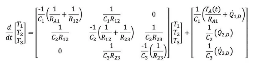
The second step was to derive the governing equation of the nodal network outlined in Figure 1. Two relevant governing equations were pertinent: Conservation of energy (i.e., an energy balance) and the thermal equivalent of Ohm’s law. These two governing equations were applied to each node and resistance, respectively. Ohm’s law assumes a linear relationship between a temperature difference and heat transfer rate, which is valid for heat conduction and convection applications with constant thermal conductivities and convective coefficients, respectively. Here, the 6 unknown variables were the 3 hardware nodal temperatures (T1, T2, T3) and 3 heat transfer components between nodes (QA1, Q12, Q23). TA is defined by a column vector of known values at all times and represents the boundary condition of the nodal network. By substituting the thermal resistances into the nodal energy balance equations, the network formulation was expressed analytically as a system of first-order linear ordinary differential equations (ODEs).
Numerical Formulation
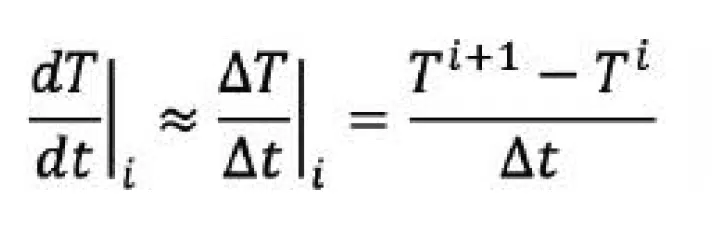
The finite difference approximation of the derivative dT⁄dt is derived from a Taylor series expansion of the function T(t) about point ti [4]:
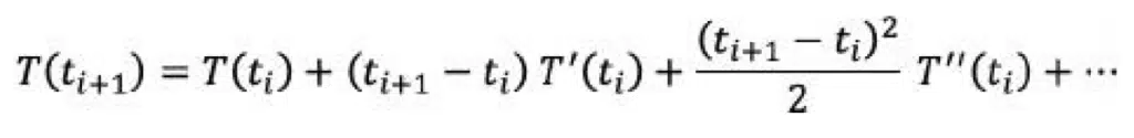
Rearranging the equation and expressing higher-order terms as O(∆t),
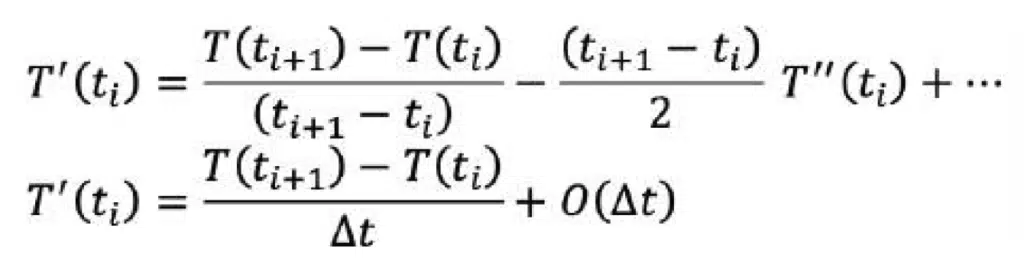
By neglecting O(∆t), the first derivative is expressed numerically in the forward Euler explicit method as:
Therefore, the third step was to express the 6 unknown variables in the forward Euler explicit finite difference formulation. A time step of ∆t=20 seconds was selected, which was more than an order of magnitude less than the upper limit for numerical stability. Considerations regarding numerical accuracy, which is dependent on the method’s truncation error and time step, and numerical stability, which is dependent on the governing equation’s eigenvalues, are discussed in Ref. [1]. All 6 equations below were necessary to define the numerical model.
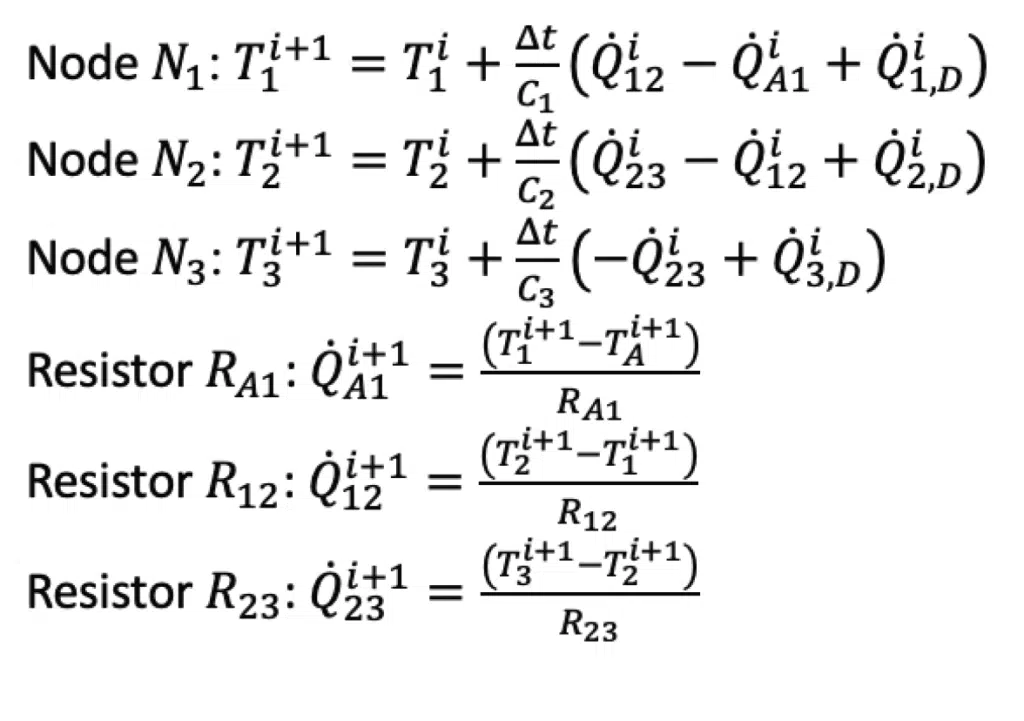
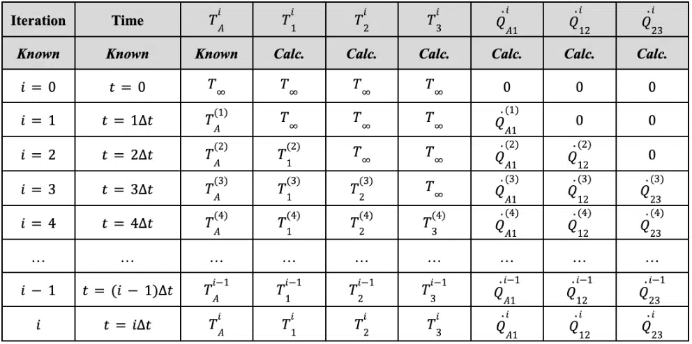
The numerical method is visually represented in Table 1 and illustrates the diffusion of heat through the nodal network from an initial perturbation in the ambient temperature, TA(1). This tabular representation can be easily implemented into a spreadsheet. With the 6 variables expressed in finite difference format and a time step selected, the functional numerical model was functional.
Numerical Model Validation and Calibration to Experimental Data
The fourth step was to validate the numerical model prior to calibrating it to the experimental data. This step was motivated by the fact that it was possible to have a functioning numerical model that did not accurately model the transient thermal response of the nodal network due to an erroneous governing equation, assumption, or numerical formulation. The model was validated by constructing the same nodal network in Icepak (ANSYS) using the same input parameters. The same nodal temperature responses were observed in Icepak, validating the construction of the numerical model [1].
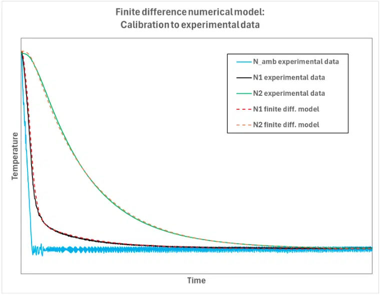
The fifth step was to calibrate the numerical model to the experimental data. This was accomplished by macroscopically matching the 6 R and C input parameters to the experimental data by trial and error. This resulted in the following input parameters to be determined: RA1=0.015°C/W , R12=0.4°C/W , R23=2.0°C/W, C1=30,000 W-s/K , C2=8,000 W-s/K , C3=3,000 W-s/K. Nodal heat dissipations were zero for the “dead mass” hardware data collection: Q1,D=0 W , Q2,D=0 W , Q3,D=0 W. Due to U.S. export control restrictions on technical data, temperature data are presented in Figure 2 qualitatively, not quantitatively, for a simplified, two-re-sistor formulation. Contrary to Figure 2, it is recommended to collect data using the hot soak temperature extreme in order to bake out any entrapped moisture within the hardware [5].
Motivation: Efficient Environmental Testing
The sixth and final step was to make use of the numerical model. The advantage of having characterized the transient thermal response of the hardware was that it enabled the development of time-efficient environmental chamber temperature profiles for environmental stress screening (ESS) of the hardware. ESS typically involves two thermal tests: Temperature cycling (TC), in which the hardware is cycled multiple times between temperature extrema, and burn-in (BI), in which the hardware is elevated to the hot soak temperature for an extended duration. Both tests are intended to detect latent infant mortality in the hardware’s electronics by conducting functional and performance tests before and after ESS. Test parameters, such as temperature extrema and number of cycles, are defined by hardware requirements and are typically derived from MIL-STD-810, MIL-HDBK-781, or SMC-S-016 in defense applications [6][7][8]. Typically, both thermal operations are required and combined into a single test, with burn-in preceding temperature cycling.
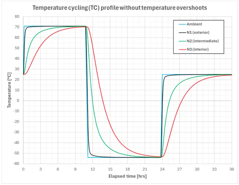
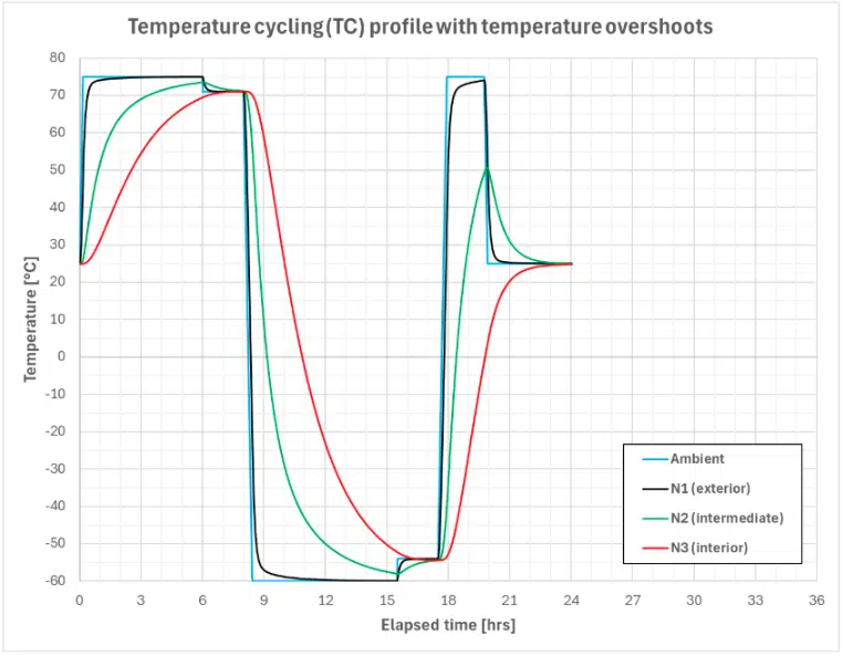
The value of performing a transient thermal characterization of a hardware system is in understanding how the hardware, in its simplified nodal network representation, will respond to any environmental stimulus. This enables the thermal engineer to incorporate small temperature overshoots during thermal ESS operations, which allow for time-efficient temperature profiles. As an illustrative example, two temperature profiles were examined: without temperature overshoots and with temperature overshoots. In both profiles, a -54°C cold soak temperature and a +71°C hot soak temperature was assumed, each with a dwell time duration of 1 hour.
The temperature profile outlined in Figure 3 does not incorpo-rate any temperature overshoots. In this profile, the hardware achieved its 1-hour hot soak after approximately 11 total elapsed hours, its 1-hour cold soak after approximately 24 total elapsed hours, and its return to room temperature after approximately 36 total elapsed hours. This profile represented the shortest total test run time possible without a thermal characterization of the hard-ware. It also required continual user monitoring of all tempera-ture data (by a machine or human) to determine when to switch the chamber temperature setpoint between extrema. In short, the temperature profile without overshoots took approximately 36 hours of environmental chamber run time.
In contrast, the temperature profile outlined in Figure 4 made use of the hardware’s thermal characterization by incorporating small temperature overshoots. Temperature overshoots entail operating the environmental chamber at more extreme temperatures to expedite steady-state conditions at each soak temperature. In this profile, the hardware achieved its 1-hour hot soak after approximately 8 total elapsed hours, its 1-hour cold soak after approximately 17.5 total elapsed hours, and its return to room temperature after approximately 24 total elapsed hours. By comparing temperature profiles, the profile incorporating temperature overshoots enabled a 33% reduction in total chamber run time, corresponding to 12 hours of time savings. This simple example demonstrates the utility of performing a thermal characterization of a hardware system to expedite ESS testing. In short, the thermal characterization enabled accurate hardware responses to temperature overshoot conditions.
One final caveat regarding the nodal network is that the quantitative value of the convective resistance RA1 was dependent on the internal airflow conditions within the environmental chamber and may vary based on specific chamber. Hence, it is recommended that experimental data be collected using the same environmental chambers and test setup as expected during ESS testing—for example, the quantity and layout of hardware systems within a single chamber.
Conclusion
This manuscript outlined a methodology for performing a transient thermal characterization of a hardware system with a finite difference model. The finite difference formulation presented herein is straightforward to understand and easy to implement on a spreadsheet. The reader is encouraged to develop his/her own spreadsheet applying the numerical model as illustrated in Table 1. The significant time savings realized by thermally characterizing hardware were demonstrated by comparing temperature profiles with and without overshoots. With the ever-growing need for cost and schedule efficiency, identifying ways to strategically reduce test time while maintaining technical integrity is paramount [9].
References
[1] A. Lozano, “Thermal Characterization Testing with a Three-Resistor Finite Difference Model,” IEEE 41st Annual Semiconductor Thermal Measurement, Modeling & Management Symposium (SEMI-THERM), San Jose, CA, March 2025, www.ieeexplore.ieee. org/document/10970672/
[2] F.P. Incropera et al., Fundamentals of Heat and Mass Transfer, 6th ed., John Wiley & Sons, 2007.
[3] R.K. Wilcoxon, “Tech Brief: Thermocouple Attachment,” Electronics Cooling Magazine, September 2024, www.electronics-cooling.com/2024/09/tech-brief-thermocouple-attachment/
[4] P. Moin, Fundamentals of Engineering Numerical Analysis, 1st ed., Cambridge University Press, 2001
[5] J.S. Wilson, “Moisture permeation in electronics,” Electronics Cooling Magazine, May 2007, www.electronics-cooling.com/2007/05/moisture-permeation-in-electronics/
[6] MIL-STD-810H with Change 1, “Environmental Engineering Considerations and Laboratory Tests,” U.S. Department of Defense, 18 May 2022
[7] MIL-HDBK-781A, “Handbook for Reliability Test Methods, Plans, and Environments for Engineering, Development, Qualification and Production,” U.S. Department of Defense, 1 April 1996
[8] SMC-S-016, “Test Requirements for Launch, Upper-Stage and Space Vehicles,” U.S. Air Force Space Command, 5 September 2014
[9] A. Lozano, “Thermal analysis methodology best practices,” Electronics Cooling Magazine, September 2024, www.electronics-cooling.com/2024/09/thermal-analysis-methodology-best-practices/