
Component reliability testing can lead to an inherent disagreement in what different people hope to see from the results. Designers who want to use the components hope that no components fail during qualification testing to verify that they meet the reliability requirement. In contrast, analysts who characterize the reliability of the components need a sufficient number of failures to establish confidence in the reliability statistics that are calculated. If a component is robust enough to pass a qualification test with no failures, the only way to satisfy both groups is to continue to test components well beyond the level needed for them to be qualified. This solution is generally not preferred by those who are responsible for paying for the additional testing.
Since the people responsible for paying for things generally get their way, statisticians should not expect that testing will always continue as long as they might hope. The question that arises then is, “If nothing fails in a test, can we draw statistically relevant conclusions from it?” Since this column is part of an ongoing series entitled ‘Statistics Corner’, one might suspect that the answer is yes.
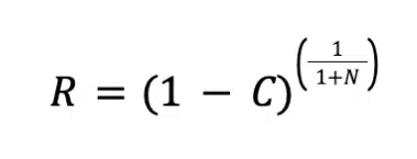
The approach described here uses the Bayes formula, as described in Reference 1. The Bayes formula defines the relationship between reliability, R, confidence level, C, and number of samples, N as:
Readers may recall a previous article in this series in which the Bayes formula was used, along with the Weibull distribution, to establish a method to demonstrate the same reliability by increasing test time/cycles in order to justify reducing the number of test samples (Reference 2). That analysis required that the Weibull shape factor of the population be estimated and equated to two tests having the same confidence level. In the approach described in this article, one defines the appropriate confidence level for the application and the number of test samples determine what reliability is demonstrated for the test conditions, in which no failures occur.
For example, Reference 3 reviewed the results from a set of three test phases in which electronic components were subject to thermal cycling aimed at inducing the formation of tin whiskers. Tin whiskers are small crystalline structures that can grow out tin materials and potentially cause electrical failures, since they can lead to electrical shorting between adjacent metal surfaces. The testing summarized in Reference 3 included three phases of testing that included 13 different component types, 7 different solder pastes, and 10 different solder finishes with a total of over 6800 individual components. All components were subjected to at least 3600 thermal cycles of -55° to +125°C, with the longest test extending to over 4300 cycles. Other than the TSOP-50 components, only one component type exhibited tin whiskers in one of the test phases. TSOP-50 components have Alloy 42 leads that have a low coefficient of thermal expansion (CTE). CTE difference within an assembly generates thermal stresses in the plating, which are known to induce tin whiskers. Since the vast majority of test combinations had no tin whiskers by the end of testing, Bayes formula was used to quantify the reliability demonstrated by the testing.
Enjoying this article?
Subscribe to Electronics Cooling for practical, engineer-focused insight on today’s thermal management challenges—plus immediate access to new digital magazine issues.
Subscribe here →
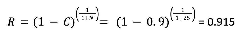
The analysis used a confidence level, C, of 90% to estimate the reliability. This value, along with the number of samples that completed a given test without tin whisker formation, was used to determine the reliability of the population. For example, a total of 25 samples of the test combination of BGA-225 (a 225-lead ball grid array component) with SAC305 solder finish and SAC396 solder paste completed 3600 thermal cycles with no tin whiskers found. With these results, the test showed a reliability of 92% for components when subjected to 3600 thermal cycles, at a 90% confidence level. The calculation used to find this result is shown below.
Other test combinations included significantly more samples, which increased the reliability estimate – but not by a huge degree. For example, some combinations included as many as 150 samples; this 6x larger sample size only increased the reliability estimate to 98%.
In an ideal world, reliability tests include enough samples and sufficient failures that we can characterize the population with a statistical function, such as a normal distribution or a Weibull distribution. However, if testing stops without any failures, we can use the approach based on the Bayes formula to quantify the results in terms of a reliability for the given confidence level.
References
[1] Lipson and Sheth, “Statistical Design and Analysis of Engineering Experiments”, McGraw-Hill, 1973
[2] R. Wilcoxon, “Statistics Corner: Modifying Sample Size”, Electronics Cooling Magazine, Summer Issue, April 2025, pp. 27-30
[3] D. Hillman, “Using The Pb-Free Solder Reflow Process as a Tin Whisker Risk Mitigation Protocol: A Statistical Assessment”, SMTAI Conference Proceedings, Chicago IL, October, 2025.