Introduction
As single-component heat dissipations in electronics cooling are increasing, air cooling is not always up to the task and is being replaced by liquid cooling. Key differences between air cooling and liquid cooling are a much higher heat transfer coefficient, higher pressure drop and much lower fluid heating. This article investigates the use of correlations to get some quick ballpark estimations of heat transfer coefficient and pressure drop. This can be a great time saver in thermal architecture and to get a viable starting geometry for further CAD (Computer Aided Design) CFD (Computational Fluid Dynamics) based design optimization. The article is based on a paper by the author presented at THERMINIC 2025 [1].
Correlations
When a fluid flows over a wall, the effect of the wall on the temperature and velocity of the fluid is limited to a thin adjacent layer, the boundary layer. The Reynolds number is a dimensionless number relating the thickness of the viscous boundary layer to a reference dimension. The Nusselt number is a dimensionless number relating the thickness of the thermal boundary layer to a reference dimension. The relative thickness of the thermal to the viscous boundary layer is a function of the Prandtl number, a dimensionless fluid property combining viscosity and thermal properties. For air, viscous and temperature boundary layers have a similar thickness. In all other fluids except liquid metals, the viscous boundary layer is thicker than the thermal boundary layer. Historically, heat transfer coefficients are calculated from Nusselt, Reynolds, Prandtl correlations, and pressure drop is calculated through a Reynolds number related loss coefficient.
Definitions of Nusselt, Reynolds and Prandtl numbers are given in equation (1), (2), and (3).
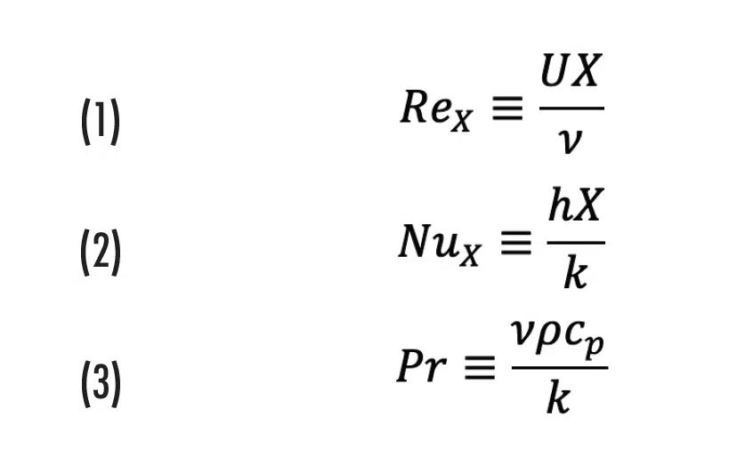
Nomenclature: U: fluid velocity (m/s), X:reference dimension (m), ν kinematic viscosity (m2/s), h heat transfer coefficient (W/m2/K), k fluid thermal conductivity (W/m/K), ρ fluid density (kg/m3), cp fluid specific heat (J/kg/K)
The advantage of using the correlations is that they are explicit formulations and hence easy to implement in a spreadsheet to give a very fast first estimate. The disadvantage is that usage critically depends on the correct identification of the type of flow a priori. If this identification is incorrect, the results of the calculation are invalid, making the use of the correlations potentially error-prone, especially for users without a formal background in fluid dynamics or in cases where geometry or fluid speed optimization is performed with a single fixed correlation equation where the flow type potentially changes with different parameter settings.
Flow Identification
Developed vs. undeveloped flow: The boundary layer thickness grows with the distance from the leading edge of the wall; in duct flow this is the entrance of the duct. Near the entrance, the boundary layers do not touch. This flow type is called undeveloped or developing and the governing length dimension is the distance to the entrance. In long ducts, boundary layers from opposing walls can grow so much that they start to touch and both adjacent and opposite walls have an influence. This is called developed flow. In developed flow, the governing dimension is no longer the distance to the entrance, but the distance between opposite walls. In non-circular ducts this distance is expressed in the hydraulic diameter Dh , given in equation 4.
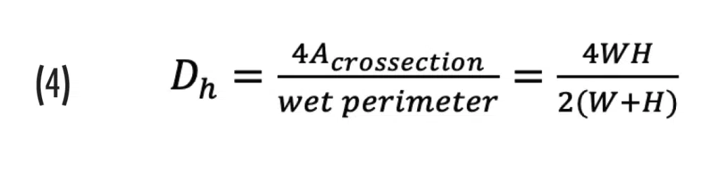
For a rectangular channel, W and H are the Width and the Height of the channel. If W>>H Dh=2H
In undeveloped flow, Nusselt and Reynolds need to be calculated with L, the length of the channel. In this paper this is indicated as NuL and ReL.
In developed flow, Nusselt and Reynolds need to be calculated with Dh, the hydraulic diameter of the channel. In this paper this is indicated as NuDh and ReDh.
Laminar vs. turbulent flow: The heat transfer coefficient quantifies the transport of heat from the wall to the undisturbed mainstream flow in the core. At low flow velocity, flow is laminar, i.e. there are no velocity components perpendicular to the wall. Heat transport to the central core is through conduction across the boundary layer thickness, averaged over the length of the wall, and can be calculated analytically. At high fluid velocities, the laminar sheets buckle and velocity components perpendicular to the wall will appear and contribute to heat transfer to the core. No analytical solution exists; turbulent heat transfer is determined empirically, and various equations exist in literature [2], [3], [4].
In undeveloped flow only the adjacent wall has an impact. The correlations for flow over a plate are the best approximation. (Equation 5) is the analytical solution for average heat transfer over a plate, (Equation 6) is a well-known correlation [2].
Laminar undeveloped:

Turbulent undeveloped:

In developed laminar flow, the average conduction length perpendicular to the wall is half the distance between the walls so the heat transfer coefficient equals:
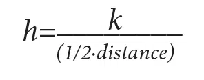
From (4) the hydraulic diameter is twice this distance Dh=2∙distance. It follows that for developed laminar flow the Nusselt number is constant and NuDh≡4. The analytical solutions align within 10%; for the constant flux boundary condition Nu=4.36 and for constant temperature boundary condition Nu=3.66.
There are many different correlations for the turbulent developed flow. One of the best known is the Dittus Boelter equation.
Laminar developed:

Turbulent developed:

The use of the value 0.4 in the exponent for Pr reflects that the flow is cooling in the Dittus Boelter correlation
Pressure Drop
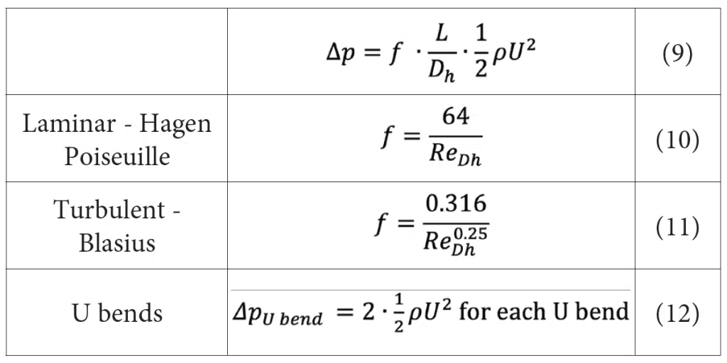
In electronics cooling, the viscous boundary layers are much thicker than the thermal boundary layers and the flow through a cooling channel is hydraulically fully developed flow. The analytical solution to the fully developed laminar case is given by the Hagen – Poiseuille equation. For the turbulent case, the Blasius equation has been shown to give good results in the electronics cooling domain [5]. In addition, also the pressure drops from ‘minor losses’ need to be considered. These are pressure drops associated with changes in the direction or speed of the flow like entry losses, exit losses, orifices or 90 degree turns. For the meandering cold plate, the pressure drop over the U bends needs to be considered. The pressure drop for flow through a duct is given by equations (9-12).
The Problem and the Workaround
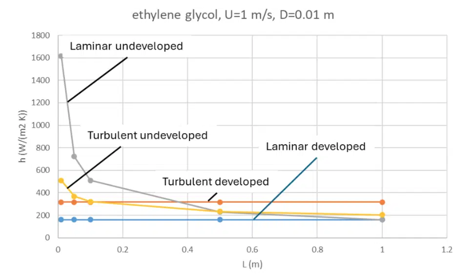
Correct classification of developing vs. developed, and laminar vs. turbulent flow is crucially important when using the Nu, Pr, Re correlations – but there are no fixed rules to differentiate them. As transitions between undeveloped and developed flow and between laminar and turbulent flow depend on geometry and experimental conditions, there is no consensus in literature as to at what exact parameter value the transition occurs. However, while differentiating between the different flow types might be difficult, choosing what heat transfer coefficient to use in engineering calculations might not be. Consider Figure 1, which shows the heat transfer coefficient for a flow of 1 m/s of ethylene glycol through a 1 cm diameter channel. The figure shows the heat transfer coefficient for different correlations at different duct lengths L. For a duct length 0.1 m (5) results in an average heat transfer coefficient h≈500W/m2/K over the length of the duct, (8) and (11) in h≈300W/m2/K, and (7) in h<200W/m2/K . The expectation is to have undeveloped laminar flow for small lengths like 0.1 m, which corresponds to the highest value of the heat transfer coefficient – in the example h≈500W/m2/K. For long lengths, the expectation is to have a developed turbulent flow and again, this corresponds to the highest heat transfer coefficient. In Figure 1: For a duct length L = 1m, (8) gives h≈300W/m2/K while (5), (6), (7), result in a lower value h≈200W/m2/K . This suggests that the difficult flow identification step can be omitted by calculating all 4 heat transfer coefficients from (5), (6), (7), (8), comparing the resulting 4 heat transfer coefficients, and using the highest value in further engineering calculations. This also makes sense from a measurement point of view: the largest effect would be the one that is most easily measured and would form the basis of the empirical correlations. A similar reasoning can be followed for the loss coefficient.
Verification of the Workaround
The workaround was tested using a commercially available CFD tool with parametric solver capabilities [6]. 210 instances were simulated, divided over 3 classes of cooling applications and 5 different fluids commonly used in the electronics cooling domain. The five liquids are pure water, 50% ethylene glycol at 20°C [7], synthetic oil at 40°C [8], plant oil at 40°C [9], and a Fluorocarbon liquid (FC) at 30° C [10]. The liquids vary by a factor 2 in volumetric heat density ρcp, a factor 9 in thermal conductivity, and a factor 41 in kinematic viscosity. Liquid properties are in Table I. The fluorocarbon is included for comparison and for historical reasons. Its present-day use is contra-indicated in view of environmental concerns and ongoing investigations on possible health hazards. The properties of air are also provided for comparison.
| Density ρ |
Specific heat cp |
Thermal conductivity k |
Kinematic Viscosity ν |
|
|---|---|---|---|---|
| kg/m3 | J/kg/K | W/m/K | m2/s | |
| Air | 1.293 | 1000 | 0.03 | 1.60E-05 |
| Water | 1000 | 4182 | 0.60 | 1.00E-06 |
| Ethylene glycol | 1082 | 3260 | 0.40 | 4.50E-06 |
| Synthetic oil | 806 | 2274 | 0.14 | 9.80E-06 |
| Plant oil | 921 | 2307 | 0.16 | 3.10E-05 |
| Fluorocarbon | 1820 | 1100 | 0.066 | 7.53E-7 |
Table 1: Liquid Properties
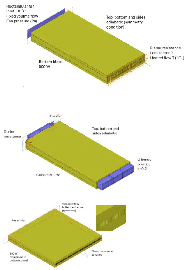
The three cooling applications are a heatsink (Figure 2-top), a meandering cold-plate (Figure 2-mid), and a microchannel plate (Figure 2-bottom). For the heatsink application, 12 different geometries were calculated with fin height 0.01 m, length range 0.05 – 0.2 m, fin gaps (channel widths) from 1 mm to 6 mm, and fluid speeds from 0.05 m/s to 1 m/s. The fins are capped with a plate to form flow channels. The meandering cold plate is 0.2 m long and has a 1.2 m long channel folded into 6 sections of 0.2 m connected by 5 non- heat transferring U-shaped bends. Channel cross-section is 0.01m x 0.01 m and fluid speeds range from 0.25 to 0.75 m/s. The microchannel geometry is closed with a plate to form channels 160 microns wide and 100 microns high with a fluid speed from 0.8 – 2.4 m/s. In total, 12 heatsink geometries were calculated for 5 liquids and 3 volume flows, the cold plate geometry was calculated for 5 liquids at 3 volume flows, and the microchannel geometry was calculated for 5 liquids and 3 volume flows, totaling 210 cases in the electronics cooling domain.
CFD Boundary Conditions and Output Parameter Extraction
The devices are situated in a solution domain with open boundary conditions at the inlet and outlet. The domain boundaries that are perpendicular to the direction of flow coincide with the top, bottom and sides and are modelled as adiabatic. Heat is applied at the bottom block of the device. A rectangular fan at the inlet of the solution domain provides the flow at an inlet temperature of 0 ° C. The pressure drop over the device is the calculated static pressure of the fan. A planar fluid resistance with loss factor = 0 is positioned a small distance downstream from the assembly. With loss factor = 0 this resistance has no impact at the flow, but it enables easy extraction of the average fluid temperature exiting the heatsink. The average fluid temperature through this planar resistance is the heated fluid temperature, Theated. This was compared to the expected value as per equation (13) and aligned well. The heated fluid temperature is subsequently used to calculate the average heat transfer coefficient for the CFD simulations using Equation (14):
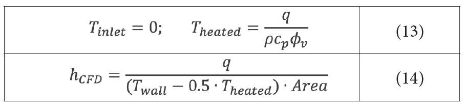
In (13) ϕv is the volume flow (m3/s). In (14) the ‘Area’ is the ‘wet’ area inside the cooling channel, and the wall temperature is taken as the volume averaged temperature of the device. The thermal conductivity of the solid material is taken as 3900 W/m/K (10 x copper) to avoid errors due to temperature non-uniformities.
Results
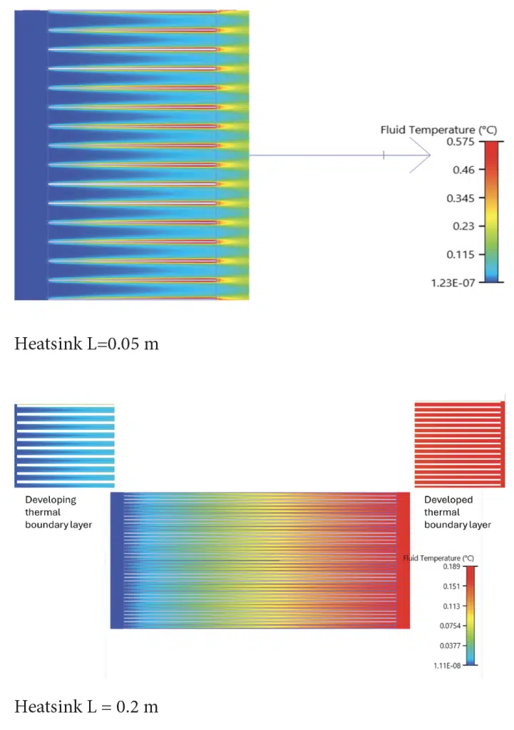
The fluid temperature distribution of two heatsink cases is shown in Figure 3. The short heatsink with L=0.05 m presents with temperature differences over the gap between the fins; the fluid adjacent to the fins is warmer while the core remains cold – this demonstrates undeveloped thermal conditions. In contrast the longer heatsink has no temperature gradient over the gap between the fins at the fluid exit at L=0.2, the flow is thermally developed.
Of the 210 cases, 59% had heat transfer coefficients associated with developed turbulent flow, 18% with developed laminar flow and 23 % with undeveloped laminar flow. There were no cases associated with turbulent undeveloped flow. For the pressure drop, 77% followed the laminar model (Hagen Poiseuille) and 23% the turbulent model (Blasius). Figure 4 compares the ratios of CFD values to separate correlations and to taking the maximum. The results demonstrate that using a single fixed heat transfer coefficient correlation can be wrong up to a factor 35. Taking the maximum calculated value performs markedly better, calculating 75% of the cases to a factor 2 or better and the remaining 25% to within a factor 3. Likewise the ratios for the pressure drop demonstrate that the strategy of taking the maximum reduces the pressure drop underestimation from a maximum of factor 70 to a maximum of about factor 5, with 75% of the values between a factor 0.8 and 2. Regression of CFD values vs. maximum value of the correlations is shown in the full paper [1]. The regressions have a slope around unity and intercepts below the regression error, providing alternative proof validating the work around.
The difference in absolute values between CFD and correlations is still considerable. This difference is due to a difference in form factors (electronics cooling applications have lower length/diameter ratios), and accuracy errors in graphing on double-logarithmic paper [11]. The explicit formulation of the correlations provides a low resource very fast method to get to a viable geometry that is likely to be overdesigned. This geometry can subsequently be used for further CFD based optimization.

transfer coefficients, bottom: pressure drops.
Conclusion
In liquid cooling of electronics, Nusselt, Prandtl and Reynolds correlations can be used for a fast estimation of heat transfer coefficient and pressured drop to be used in engineering calculations. A disadvantage of the use of the correlations is that the choice of what correlation to use crucially depends on the correct classification of the flow as undeveloped vs. developed, and laminar vs. turbulent. Classification depends on fluid properties, fluid speed and mechanical dimensions. Therefore, flow classification is needed for each design iteration in a correlation-based model where these parameters are varied, which is cumbersome and a potential source of error. Flow classification is unnecessary in CFD simulations, but these are more time and computational resource intensive. This article proposes a way to avoid the classification step by calculating the heat transfer coefficient for the 4 different classes (developed/undeveloped flow and laminar/ turbulent flow) and taking the highest value. Likewise for the pressure drop the highest value of the loss coefficient between the laminar and the turbulent case is taken. Taking the maximum value out of a group is a standard spreadsheet function that is easily added to the correlation formulations; therefore, the new method enables optimization of geometries and fluid speed in a spreadsheet without the classification step at each design iteration. The method was validated with CFD against 210 CFD simulations over a wide range of electronics cooling applications. Results demonstrate that ‘using the highest value’ aligns much more closely to CFD than picking one correlation and sticking to it, what is essentially what happens if a single correlation is used during the optimization iterations. In absolute sense the correlations underpredict the CFD values by up to a factor 3 due to form factor differences and historical graphing inaccuracies, so the use of CFD for more accurate details is still indicated. The proposed way of working is to use the correlations and the ‘take the highest’ strategy to come to a viable design and use this as the starting point for subsequent CFD optimization.
References
[1] W. Luiten, “Heat Transfer Performance Modelling for Liquid Cooling of High-Power Electronics,” 2025 31st International Workshop on Thermal Investigations of ICs and Systems (THERMINIC), Naples, Italy, 2025, pp. 1-6, doi: 10.1109/ THERMINIC65879.2025.11216924.
[2] Wong, H.Y., 1977. Handbook of essential formulae and data on heat transfer for engineers. London: Longman
[3] F. Incropera, and D. DeWitt, 1996. Fundamentals of Heat and Mass Transfer. John Wiley & Sons, Inc., New York City, New York, 4th Edition edition, (1996)
[4] Bejan, A. (2013) Convection Heat Transfer. 4th Edition, Wiley, NewYork. http://dx.doi.org/10.1002/9781118671627
[5] McKeon, B. J.; Zagarola, M. V; Smits, A. J. (2005). “A new friction factor relationship for fully developed pipe flow” . Journal of Fluid Mechanics. 538. Cambridge University Press: 429–443. doi:10.1017/S0022112005005501.
[6] https://www.siemens.com/en-us/products/simcenter/fluids-thermal-simulation/flotherm/
[7] Ethylene glycol properties, engineering toolbox, www.engineeringtoolbox.com/ethylene-glycol-d_146.html, retrieved July 2025.
[8] Datasheet Shell SX5, https://industrialfluidsmfg.twinoils.com/Asset/Shell%20Immersion%20Cooling%20Fluid%20S5%20X.pdf,
[9] DatasheetNature Cool, https://www.cargill.com/bioindustrial/doc/1432245644639/naturecool-2000-tds.pdf, retrieved July 2025
[10] Fluorinert FC3283 Technical Data | July 2015 (3m.com) retrieved July 2025
[11] Dittus, F. W. and Boelter, L. M. K., (1930) Heat transfer in automobile radiators of the tubular type. University of California Publications in Engineering, 1930,2,443461