Introduction
Parametric design plots are commonly used in early thermal architecture studies to understand sensitivity across the design space, often resulting in the selection of a single-point solution that achieves a key design objective. For example, the size of a passively cooled consumer electronics device may be selected such that it achieves the required thermal design power (TDP) in a standard room temperature environment.
This is an effective thermal design approach to obtain a quick binary result. The example consumer electronics device will either meet or not meet its requirement at any point in the design space.
So, when do we need to consider expanding beyond this approach? It is a good idea to consider your options when you expect variation in your inputs, or when a customer is interested in understanding the percentage of time a thermal requirement will be achieved in the real world.
We will introduce a Monte-Carlo approach that will enable you to explore the robustness of your thermal design. This approach can be applied to data centers, aerospace, automotive, consumer electronics, etc.
Parametric Design Plot
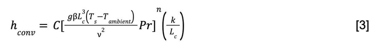
We will leverage the consumer electronics device that we explored in a previous calculation corner [1]. The device has the form factor of a mobile phone (see Figure 1), with a coefficient of thermal spreading (CTS) of 0.55, and a 1.6W use case. Note that the CTS represents a performance metric that compares the real versus ideal power dissipation of the mobile device as defined here [9]. The surface temperature of the device must remain between 10°C and 45°C when in a 25°C ambient environment. If the device drops below the lower temperature limit, its voltage may drop below its typical operating point and cause a brown out; if it exceeds the upper limit, it will be throttled to maintain user comfort.
Now let’s write the steady-state energy balance for the mobile device (equation 1), where heat rejection is dominated by natural convection & radiation. Qinput is the heat generated in the device, hconv is the convective heat transfer coefficient, A is the external surface area, CTS is the coefficient of thermal spreading, Ts is the surface temperature, Tambient is the ambient temperature, ε is the emissivity, σ is the Stefan Boltzmann constant, and F is the view factor. This equation can be simplified by linearizing radiation using equation 2, assuming an emissivity of 0.85 and a view factor of 1.0.
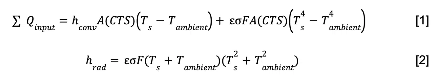
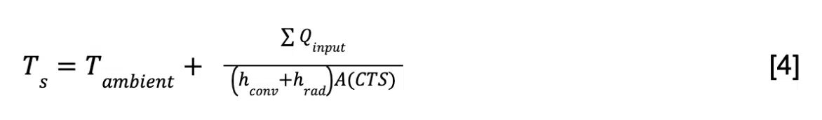
The natural convection heat transfer coefficient (hconv) can be estimated using the empirical correlation provided in equation 3, where k is the thermal conductivity of fluid, Lc is the characteristic length of the body, g is the acceleration of gravity, β is expansion coefficient, v is kinematic viscosity, Pr is the Prandtl number, and C and n are empirical constants. We will assume the fluid properties of air and use coefficients C and n of 0.59 and 0.25 that are suitable for a vertical plate [2].
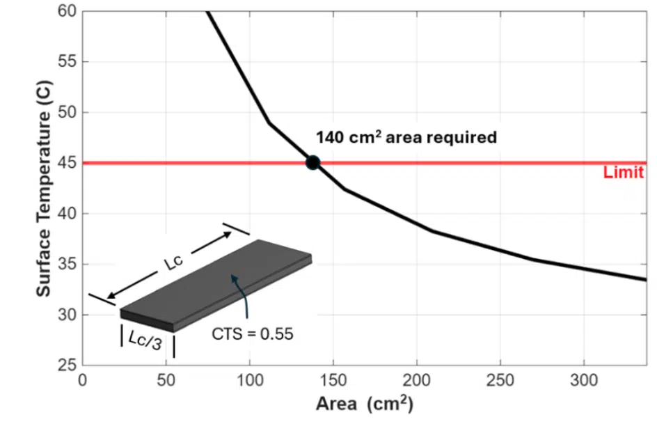
Rearranging the energy balance enables us to solve for the surface temperature via equation 4. Note that an iterative solution process is required as the heat transfer coefficients are dependent on the surface temperature.
The parametric design plot in Figure 1 is generated by calculating the surface temperature as a function of the device area. It indicates that an area of 140 cm2 is required for the device to meet the desired 1.6W use case without throttling. Parametric design plots like this are commonly used and can be excellent tools, especially in established fields where a single-point design has been validated to bound device usage. The design point in this example is a 25°C natural convection environment with a power of 1.6W.
environment
Monte Carlo for Indoor Usage
Let’s now take the mobile device with a 140 cm2 area that we determined from the parametric design plot and introduce real-world variability.
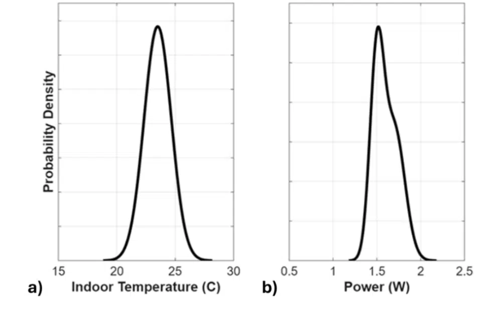
The ambient temperature in controlled indoor environments is typically maintained between approximately 20°C and 27°C, per ASHRAE standards [3]. We will assume that the ambient temperature follows the normal distribution illustrated in Figure 2a. The interested reader can find additional indoor temperature measurements in [4].
It is also common for the power of electronic components to vary from part-to-part. This can be a function of manufacturing tolerances, process changes, different leakage behavior, etc. While one could control this variation with techniques such as part binning, we will assume the power needed for our components to deliver the desired use case follows the bimodal normal distribution illustrated Figure 2b.
We now have everything we need to run a simple Monte-Carlo analysis and evaluate the robustness of our single-point design when exposed to real-world indoor environments.
But wait, what is a Monte-Carlo analysis [8]? Monte-Carlo analysis simply solves our existing thermal model (equation 4) but repeats the calculation to predict many embodiments of the solution, each with inputs that are randomly drawn from the statistical distributions of our input parameters (Figure 2). See Figure 3 for a block diagram of the Monte-Carlo solution process.
Each embodiment in a Monte-Carlo analysis is referred to as a draw. The total number of draws needed for a Monte-Carlo analysis will depend on the specific problem, often landing between one thousand and one million.

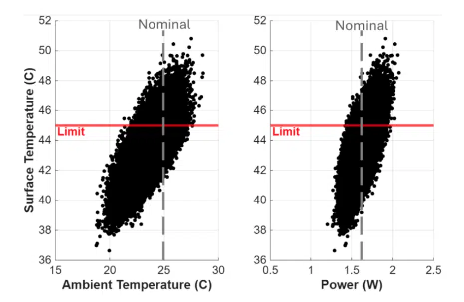
Now let’s evaluate our device using the Monte-Carlo approach with 100,000 draws. The results are illustrated in the scatter plot provided in Figure 4. Unlike our original parametric design plot that focused only on a single point in the design space, we see variation in the device surface temperature that stems from the introduction of real-world variation in our input parameters. Each marker in Figure 4 represents one draw from the Monte-Carlo simulation. Figure 4 provides a visual representation of the surface temperature variation as a function of each of our independent input parameters. The minimum, average, maximum and standard deviation of surface temperatures predicted by the Monte-Carlo are 37°C, 43°C, 50°C, 1.6°C respectively.
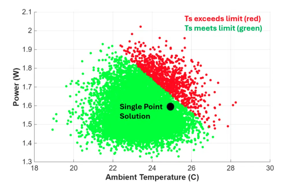
The results are replotted in Figure 5 to illustrate the combination of input parameters that will lead to system throttling. First, it is easy to see the real-world variation that occurs around our original design point. We also see that our device exceeds its thermal limit 9% of the time, specifically when the ambient temperature and/or power exceed our assumptions in the original design point.
Monte Carlo for Indoor and Outdoor Usage
Let’s add one more layer to this example to illustrate ways that you can expand your Monte-Carlo to consider more complex interactions. Specifically, let’s consider what happens if our device is used both indoors and outdoors.
Enjoying this article?
Subscribe to Electronics Cooling for practical, engineer-focused insight on today’s thermal management challenges—plus immediate access to new digital magazine issues.
Subscribe here →
Human activity pattern studies [7] indicate that people spend most of their time indoors. Thus, we will assume that the device is indoors 90% of the time, and outdoors the remaining 10%.
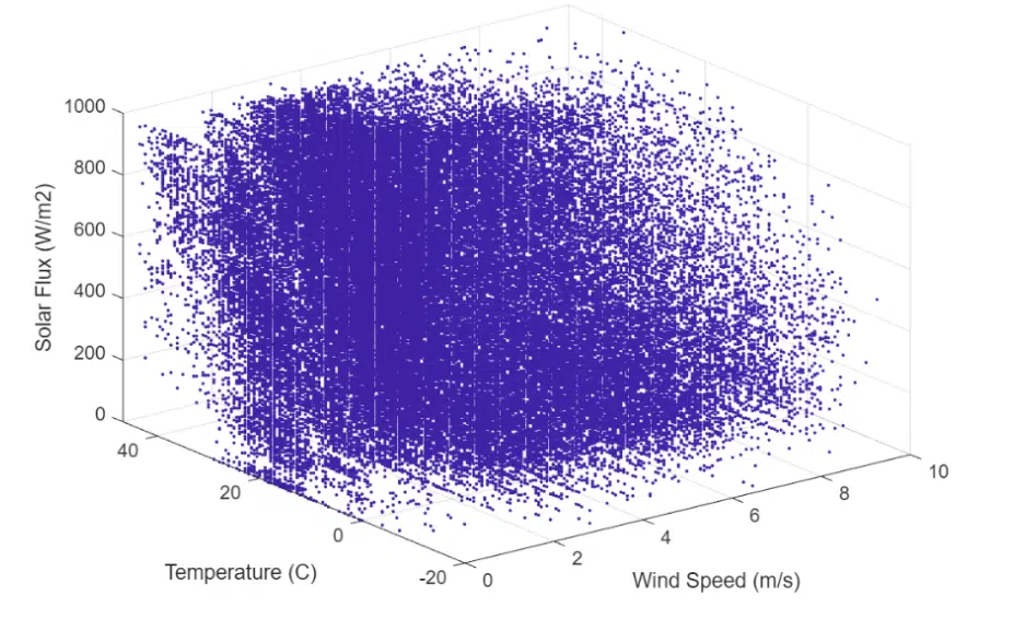
Outdoor environmental inputs typically consist of the temperature, windspeed, and solar heat flux. These values are typically not independent. For example, you may expect increased windspeeds and solar loads when the ambient temperature is high. Luckily there is a wealth of meteorological data available that we can leverage to understand these interdependences [5] [6]. For this study we will leverage real meteorological readings over a 5-year period in the cities of Phoenix, Chicago, New York, and Los Angeles. The point cloud of our outdoor data is provided in Figure 6. For our Monte-Carlo we will simply randomly select points from this dataset when outdoors.
Now that we have our outdoor environment defined, we just need to make a few modifications to our model. First, an additional heat source is needed to account for the solar radiation. This is included by multiplying the solar heat flux by the area of one side of the device (assuming horizontal orientation) and the solar absorptivity (assumed to be 0.85).
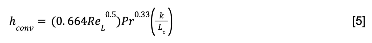
We also need to adjust the outdoor convective heat transfer coefficient to a forced convection relationship that accounts for wind. We will use the laminar flat plate correlation in equation 5, where ReL is the Reynolds number calculated at the characteristic length.
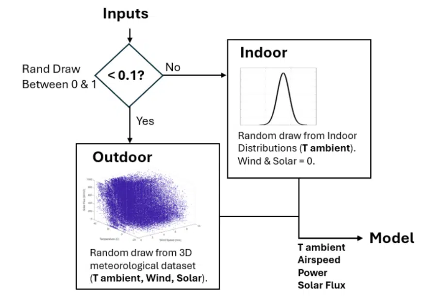
We now have everything we need to re-run our Monte-Carlo analysis for indoor and outdoor usage. We can determine our model inputs using the decision tree illustrated in Figure 7 and then solve equation 4 for the surface temperature.
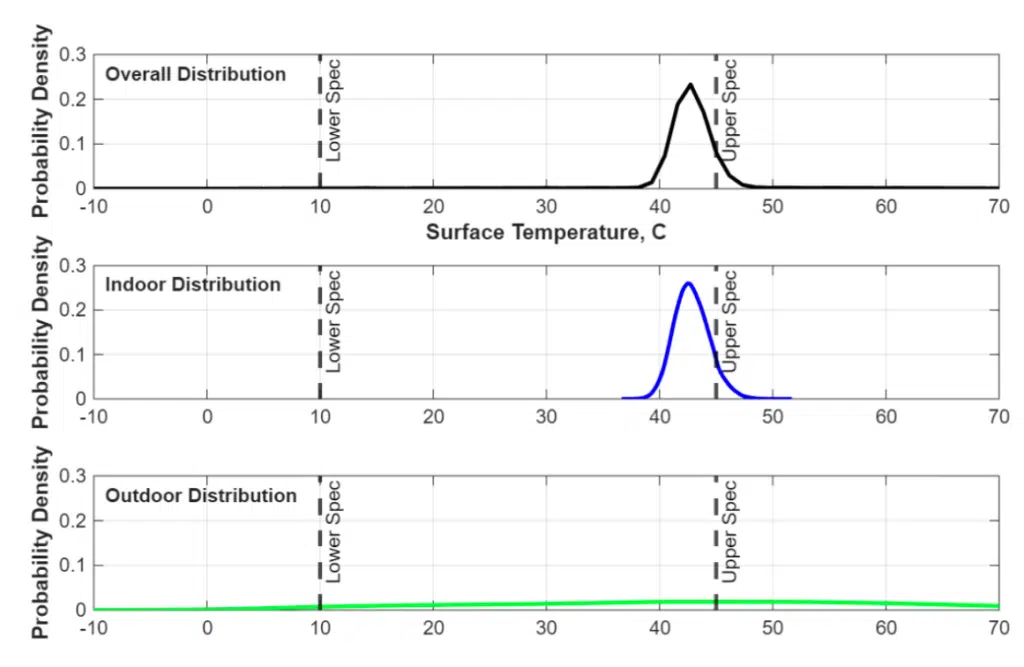
The resulting surface temperature distribution is illustrated in Figure 8. The overall distribution closely follows the indoor usage distribution. This is expected given the high percentage of time users spend indoors. However, the addition of outdoor usage extends the tails of the distribution. This captures low temperature conditions that will cause brownout, as well as higher temperature extremes in hot geographic locations with solar heating.
The inclusion of outdoor usage increased the likelihood of our device being thermally limited from 9% to 13%. While the overall impact may not seem large, it does indicate that our device may exhibit unacceptable performance when outdoors, since it throttles in ~40% of outdoor use cases.
Conclusions
A comparison between the single-point design solution and the Monte-Carlo solution is summarized in Table 1. Both approaches have their place in the thermal designer’s toolbox. Single-point design solutions are simple, can often be completed on the back of an envelope, and provide a simple binary result. However, if you expect variation in the real-world, the Monte-Carlo approach provides additional insights into design robustness.
As illustrated in this example, the Monte-Carlo approach provides an estimate of the likelihood that thermal design limits will be met in the real world. The approach is flexible and can be used with various input distributions, incorporate logic-based decisions trees (e.g., indoor vs. outdoor), and can be used with any type of thermal model. While a simple thermal model was leveraged in this illustration, the approach is equally valid for more complex thermal models.
| Surface Temperature | Percentage of time within design limits | |
|---|---|---|
| Single-Point Design |
45°C | 100% |
| Indoor Monte-Carlo |
Min: 37°C Avg: 43°C Max: 50°C |
91% |
| Indoor & Outdoor Monte-Carlo |
Min: -10°C Avg: 43°C Max: 100°C |
87% |
Table 1: Results comparison for solution techniques
Although we now have an understanding of Monte-Carlo analysis as a thermal design tool, it is only responsible to also acknowledge that it is not the best approach for every problem. The outputs are only as good as the inputs, so it is essential that we have confidence in our statistical inputs before jumping to a Monte-Carlo. Additionally, the approach can become computationally expensive when complex thermal models are involved. If you fall into this category and still want to understand design robustness, you can also consider a simulated design of experiments approach, reviewing telemetry from similar products, or even exploring approaches that leverage artificial intelligence models.
References
[1] Alex Ockfen, “Calculating Thermal Design Power for Mobile Consumer Electronics – Part 1”, Electronics Cooling Magazine, February 2023
[2] Frank Incropera and David DeWitt, Fundamentals of Heat and Mass Transfer, 4th Edition, Wiley (1996)
[3] ASHRAE Standard 55, Thermal Environmental Conditions for Human Occupancy, 2010
[4] NREL/TP-5500-68019, Residential Indoor Temperature Study, April 2017
[5] NOAA Online Climate Tools, https://www.ncdc.noaa.gov/cdo-web/datatools
[6] NREL Solar Database, https://docs.nrel.gov/docs/fy12osti/54824.pdf
[7] Neil Klepeis, William Nelseon, et. Al, “The National Human Activity Pattern Survey (NHAPS)”, Journal of Exposure Science & Environmental Epidemiology, 2001
[8] Bruce Guenin, “Use of the Monte Carlo Method in Packaging Thermal Calculations”, Electronics Cooling Magazine, March 2018
[9] Victor Chiriac, “A Figure of Merit for Smart Phone Thermal Management”, Electronics Cooling Magazine, December 2015